A histogram answers a narrow but useful question: how are the image’s decoded tones distributed? Use it alongside the picture to examine an edit, compare color channels or document a result without relying only on the appearance of one display.
- The tested example
- Step 1: Open the histogram workspace and choose the right source
- Step 2: Read the brightness distribution and pixel count
- Step 3: Inspect an RGB channel and reveal small peaks
- Step 4: Export the numeric data and the selected chart
- Check the result
- Troubleshooting
- Practical details
- Example sources
TESTED WORKED EXAMPLE
What this session produced
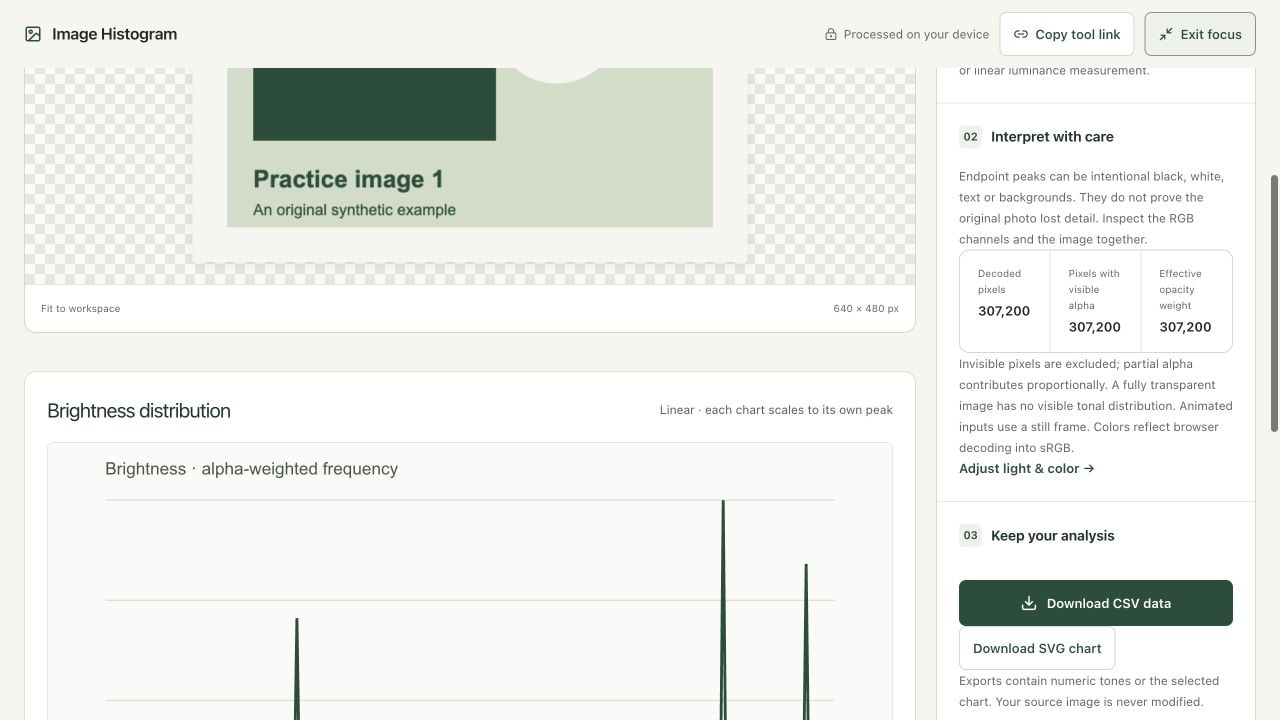
The 640 × 480 practice PNG contained 307,200 decoded pixels, all fully opaque. Its brightness mean was 187.47 and median was 216. The exported CSV contained 256 bins for each of four channels, and each channel’s opacity-weighted total was 307,200.
The screenshots were captured from the working local tools on October 7, 2026. Focus workspace gives the controls and preview more room. Each image shows the relevant visible workspace state; these are real captures, not recreated interface illustrations. Results describe these samples and settings rather than a promised outcome for every file.
Follow the worked example
Step 1: Open the histogram workspace and choose the right source
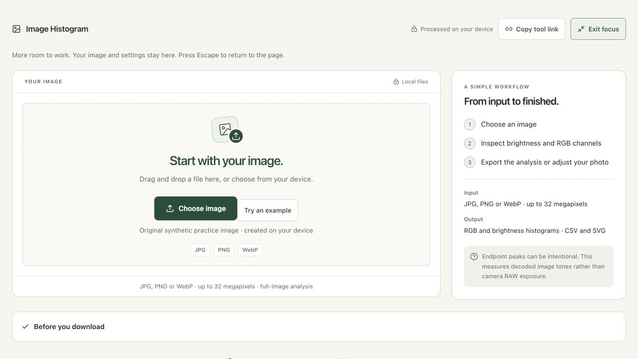
Open Image Histogram and select Focus workspace if you want more room for the controls. Choose a supported JPG, PNG or WebP, or use Try an example to follow this controlled session. Work from the file you actually need to inspect: a screenshot, an exported edit and a camera original can have different tonal distributions. This tool analyzes a decoded still image rather than a camera RAW file. It does not modify or compress the source.
Step 2: Read the brightness distribution and pixel count
Choose Try an example. The graphic is 640 × 480, so its decoded pixel count is 640 multiplied by 480, or 307,200. Leave Histogram channel on Brightness and Vertical scale on Linear. Review the chart alongside the source and the statistics below it. In this session the mean is 187.47 and median is 216. Those values describe this graphic, including its pale background, rather than a universal target for a well-exposed photograph.
Step 3: Inspect an RGB channel and reveal small peaks
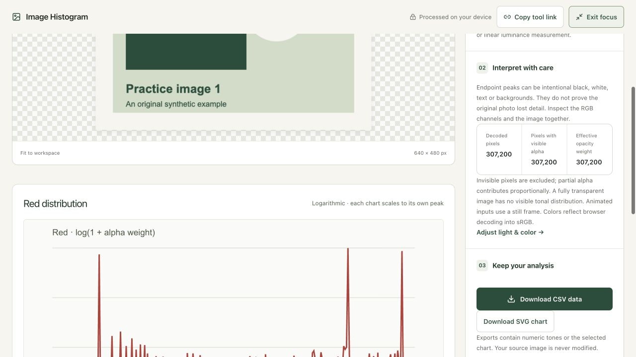
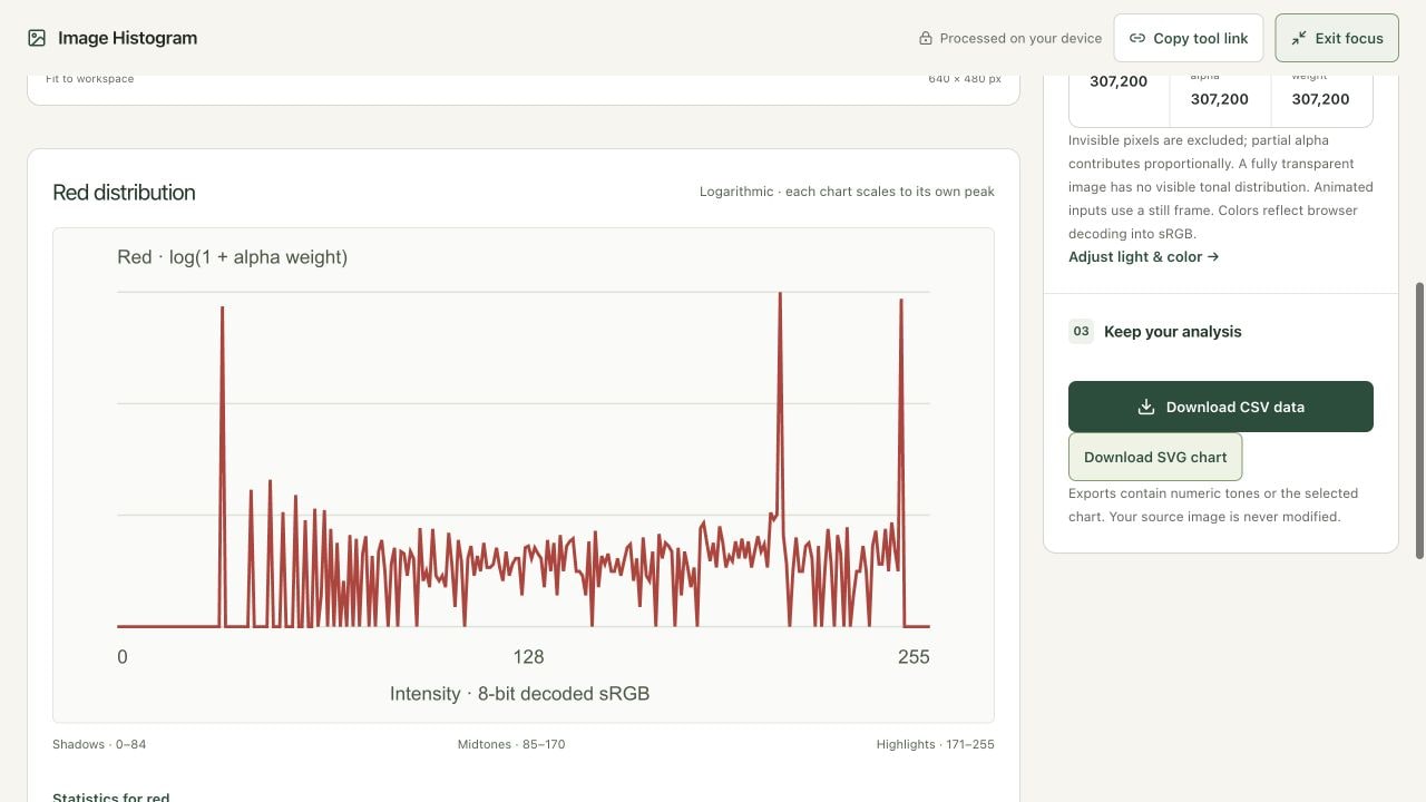
Select Red in Histogram channel, then Logarithmic in Vertical scale. The chart changes to the red values and uses log(1 + weight), making smaller populations easier to see beside large peaks. This session’s red mean is 175.78. Inspect Green and Blue in the same way when color balance is relevant. Changing the channel or chart scale changes the analysis view only; it does not recolor the picture, change its pixels or change the CSV’s underlying bin counts.
Step 4: Export the numeric data and the selected chart
Choose Download CSV data to keep all 256 bins for Brightness, Red, Green and Blue. Choose Download SVG chart to keep the currently selected red/logarithmic chart. Read the channel and scale labels before using that illustration in a report. The SVG describes a normalized display; the CSV supplies the actual opacity-weighted counts. Keep the file’s dimensions and processing context with the analysis so a later export or crop is not mistaken for the same source.
Check the result before using it
Open the CSV and confirm that intensity runs from 0 to 255 with four channel columns. For this fully opaque practice graphic, each channel sums to 307,200. A partly transparent source can have a smaller effective opacity weight. Open the SVG separately and check that its channel and scale match your selection. Neither download is a replacement image.
If the result is not what you expected
A blank distribution can be correct for a fully transparent image. A very tall spike can come from a flat background, logo or text; it does not prove the file is defective. Check the selected channel and whether the vertical scale is logarithmic before comparing charts. Convert HEIC through the dedicated converter, and use a smaller working copy only when a source exceeds the supported limits.
Background and practical details
Read position and height as different measurements
The horizontal axis is intensity: 0 is the low endpoint and 255 is the high endpoint of an 8-bit channel. The vertical shape describes how much visible image data occupies those bins. A tall peak can represent a large flat area, while a low peak can represent a small but important detail. A histogram cannot tell you where those pixels occur in the picture. Inspect the subject, background and small details together.
Adobe’s histogram reference explains intensity distributions and channel statistics. That general idea also applies here, but the calculation below is this workspace’s implementation; it should not be assumed to match every Photoshop mode or a camera’s histogram.
Understand what Brightness measures here
The workspace computes a rounded estimate from browser-decoded, gamma-encoded sRGB values: 0.2126 R + 0.7152 G + 0.0722 B. Green contributes most to that estimate. It is not a linear-light luminance calculation and does not inspect the sensor’s original exposure data. A saved JPG may already include a tone curve, edits and compression. Its histogram describes that decoded copy.
Shadows cover bins 0–84, midtones 85–170 and highlights 171–255 in this interface. These fixed ranges organize the statistics; they are not a diagnosis of whether a scene should be brighter. The displayed mean is an average weighted intensity, the median is the midpoint of the accumulated weight, and standard deviation describes spread. Two pictures can share these summaries while showing completely different subjects.
Keep transparency out of the wrong conclusion
Fully transparent pixels contribute no visible weight, even if their hidden RGB channels contain black or another color. Partially transparent pixels contribute in proportion to their alpha value. For example, a pixel with alpha 128 contributes 128/255 of a fully opaque pixel’s weight. This example explains the calculation; it is separate from the fully opaque fixture used in the screenshots.
The histogram is not the distribution after compositing the image over a white or dark background. A pale cutout edge can look different over different surfaces. Use Transparency Checker when you need to inspect actual alpha, and use the preview backgrounds to judge an intended composition. A fully transparent image has no visible tonal distribution; empty statistics are therefore expected.
Compare scales and endpoint peaks carefully
Each chart is scaled to its own peak. The highest red and blue peaks can both reach the top of the display while containing different counts. Logarithmic scaling is useful for seeing small populations, but it changes their displayed height relationship. Use the CSV for numeric comparisons, with the same dimensions and transparency treatment for both inputs.
Values at 0 or 255 can be intentional black lettering, a white background or a graphic element. Endpoint counts alone do not prove that a photograph lost highlight or shadow detail. Likewise, an empty endpoint does not prove that every important tone survived an earlier edit. Compare the actual image with its source before deciding what to change.
Use the analysis to guide a controlled next step
If an edit needs review, open Photo Adjustments, make a small change and export a separate copy. Analyze that copy alongside the original using identical channel settings. Record which export and dimensions you inspected. A fitted preview can hide small artifacts, so inspect the downloaded image at a useful scale before accepting it.
The tool checks every decoded pixel rather than sampling a few points. It accepts supported still-image inputs up to 32 megapixels, with a maximum side of 8,192 pixels and a 50 MB file limit. Browser resources still matter. Animation is represented by a decoded still frame here, not a timeline. Local image processing also does not mean that loading a website requires no network traffic; see the privacy policy for that distinction.
Example sources and screenshot notes
This session uses the original synthetic practice graphic created by Smart Image Tools. No stock photograph or personal image is involved. The numeric results are a controlled example, not a photographic exposure or quality benchmark.
Keep an untouched source and verify the actual downloaded result. If a control or result differs from this guide, send the article URL and the setting involved. Our editorial policy explains how corrections are reviewed.
Find the right tool for your image.
Explore the free workspaces, read their methods and inspect your result before sharing.
Explore image tools